A few people have contacted me about machine learning in a time series data set. These short of datasets require a little bit extra in terms of data processing, as you are trying to predict the outcome of a future data point, this means you have to obtain that data point, and classify it. For this brief example, we will look at stock market data: all_stocks_5yr.csv for the last 5 years. We have to note though, time series data is hard to predict, and there’s a lot of reasons why a stock will go up or down, not just it’s previous data points. This is merely used as an example, it’s not an endorsement that a simple application of a machine learning algorithm should be used to predict stocks. Again, this is mainly about how to process time series data for machine learning. First of all we import the following modules:

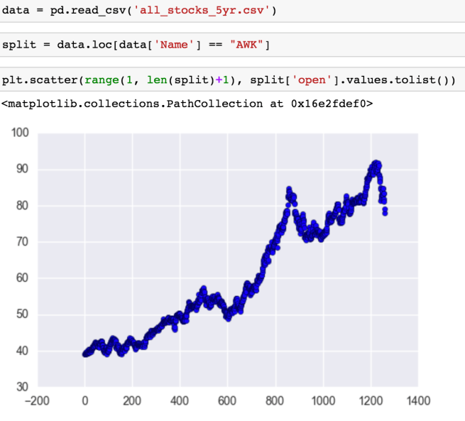
We then read the data, select a stock that we want to analyze, and plot it to get a feel for it. Note that I make a new data frame called split as opposed to writing over the original data frame:

Now with time series we usually consider rates of change. This is the difference in x and y between two different points. However, between all data points in a column, the x difference will be the same, so we will just focus on the change of y. Now I like converting the columns into lists and looping through as vectorization becomes tricky when you’re taking into account data points before and after the data point. Because of this, I like to make the columns first:

diff just means difference. Two and three means two of three data points back, and bin is short for binary meaning one for an increase over time, and zero of a decrease over time. This is where we have to define our machine learning question and tool for the time being. Predicting everything here is just too much, for this approach we will see if we can predict if the closing price tomorrow will be higher or lower than the opening price today. A simplistic binary outcome can be done using logistic regression. Now we can calculate our outcome and rates of change by the following loops:

 Notice that I had to fill the first four with none values. This is because rates of change cannot be calculated with no previous data points. We will use the dropna to get rid of these later. We now add the values to the split data frame:

We now drop all of the fields that cannot be utilized by logistic regression:

Now let’s look to see if there’s anything else that we can pull from the data. We can plot all the variables against each other using seaborn:

You can see that there’s clustering. If negative and positive points cluster together, this could be another form of classification that could be fed into the logistic regression algorithm. If a positive point falls into the parameters of the positive cluster it could be assigned a value one in a cluster column. We can chart it by the following:

Giving the following plot:

As you can see, there’s a lot of cross-over. I went through all the clusters and nothing. This is usually the case. Clustering is a machine learning project in itself and it’s a bit of a golden gift if you stumble across clean clustering. We create a set of outcomes (y), and a set of inputs (x). We then split it into test/train data, fit the logistic regression model and test it:

….. ok so it’s better than flipping a coin. We didn’t plot a training curve or cross validate, and the number of data points is low. Considering this, I ran it a few times and the results varied a lot, which isn’t a good sign, but this post is focusing on time series. Overfitting and learning curves is a different subject for another post. But we might as well apply it to see where the errors are happening. We get the logistic coefficients by the following:

We do this defining the logistic function and apply it to the data frame:

Now that we’ve calculated the logistic function for each data point, we can compare it with the actual rate of change to see where it fails:

We can now plot the failure points in the time series by looping through. If it’s positive it gets appended to one list and if it’s negative gets appended to another list:

As you can see there’s no outright failure at a particular point. And there you have it! This is how you process time series data. Of course, there’s more you can do, but now you have the basics of time series analysis, you can keep going. Ideally the outcome of this logistic regression would be a variable in a bigger machine learning algorithm that would take into account factors such as new streams etc.